This section presents the algorithms employed for the discovery of portable objects. While a comprehensive technical analysis of these algorithms is beyond the scope of this work, they are described with sufficient detail to enable understanding of their application within our framework. For in-depth technical details and formal derivations, the reader is referred to the original publications cited herein. To demonstrate the different navigators, a costmap of the Pulse Breakout room is used. This map was obtained during testing of the coverage methods. Furthermore Nav2 Macenski et al., 2020 is used for low level motion planning and execution as well as real-time control and costmap generation.
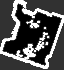
Figure 1:Initial costmap of the Pulse Breakout room used to evaluate the coverage planners.
Source
import cv2
import numpy as np
import matplotlib.pyplot as plt
import ipywidgets as widgets
from IPython.display import display

def interactive_path_slider(
    image_path,
    csv_path,
    title="Path Viewer",
    color=(0, 255, 255),
    thickness=1,
):
    """
    Visualize a path stored in CSV over an image.

    Parameters
    ----------
    image_path : str
        Occupancy map image.

    csv_path : str
        CSV with columns:
            x,y
            74,19
            75,20
            ...
    """

    plt.ion()

    # -------------------------------
    # Load image
    # -------------------------------

    map_img = cv2.imread(image_path, cv2.IMREAD_GRAYSCALE)

    if map_img is None:
        raise ValueError(f"Could not load image: {image_path}")

    # -------------------------------
    # Load path
    # -------------------------------

    path_pixels = np.loadtxt(
        csv_path,
        delimiter=",",
        skiprows=1,
        dtype=np.int32,
    )

    if path_pixels.ndim == 1:
        path_pixels = path_pixels.reshape(1, 2)

    # -------------------------------
    # Draw path
    # -------------------------------

    vis = cv2.cvtColor(map_img, cv2.COLOR_GRAY2RGB)

    cv2.polylines(
        vis,
        [path_pixels],
        isClosed=False,
        color=color,
        thickness=thickness,
    )

    # -------------------------------
    # Create figure
    # -------------------------------

    fig, ax = plt.subplots(figsize=(8, 8))

    ax.imshow(vis)
    ax.set_title(title)
    ax.axis("off")

    robot_dot, = ax.plot(
        path_pixels[0, 0],
        path_pixels[0, 1],
        "o",
        color="yellow",
        markersize=10,
    )

    # -------------------------------
    # Slider
    # -------------------------------

    slider = widgets.IntSlider(
        value=0,
        min=0,
        max=len(path_pixels) - 1,
        step=1,
        description="Waypoint",
        continuous_update=True,
        layout=widgets.Layout(width="800px"),
    )

    def update(change):

        idx = change["new"]

        x = path_pixels[idx, 0]
        y = path_pixels[idx, 1]

        robot_dot.set_data([x], [y])

        fig.canvas.draw_idle()

    slider.observe(update, names="value")

    display(slider)
plt.show()Preprocessing
Before the map can be used to plan a path, a common preprocessing algorithm can be abstracted. Coverage path planners generally use either a binary map of the free space, (free=1, occupied=0) or the polygons constructed from the boundaries of the free space.
The input to the algorithm can be any 2D image displaying the free and occupied pixels. In this case the input will be the costmap directly. First the costmap is thresholded to create a binary costmap, which is the first output.
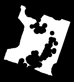
Figure 2:Binary costmap generated by thresholding the Nav2 costmap into free and occupied space.
Then using this binary costmap, the contours Figure 3 are extracted.
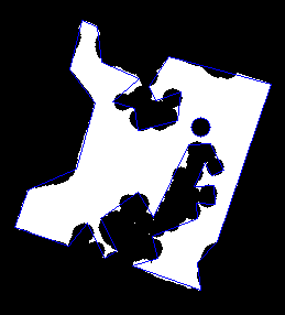
Figure 3:Contours extracted from the binary costmap representing the boundaries of free space.
Morphology-Based Skeleton Path Planner
The first implemented method, based on the work of Becoy et al., 2025, Niu et al., 2025, derives a coverage path from the morphological skeleton of the free space. See the algorithm below.
Input: Occupancy grid , robot start position
Output: Ordered waypoint segments
threshold(, lethal_threshold)
Extract contours from , group by containment into polygon groups
For each polygon group :
medialAxis() (skimage skeletonize)
skeletonToWorldCoords()
buildKDTreeGraph(, radius )
bridgeDisconnectedComponents()
findLeafNodes() (nodes with degree 1)
nearestLeaf(, )
,
While :
nearestLeafByGraphDistance(, , )
shortestPath(, , )
append to
append to , set
sanitiseWaypoints(, )
Return
The free space is extracted using the methods discussed in the previous section. The polygons are used and converted to a binary map as to not produce too many branches for the robot to navigate through. This map is then skeletonized to extract waypoints, see Figure 4.
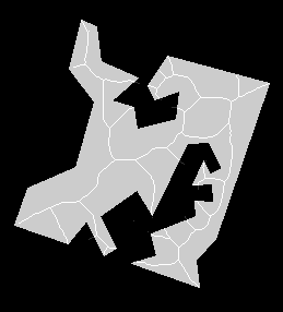
Figure 4:Morphological skeleton extracted from the free-space representation of the environment.
Once the waypoints are obtained, a graph is constructed and leaf nodes are extracted. In the graph leaf nodes are defined by their single connection to the rest of the skeleton, these are seen as endpoints of the path.
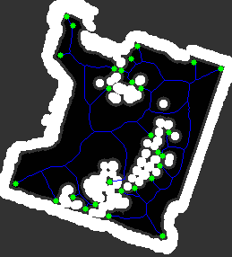
Figure 5:Leaf nodes identified on the skeleton graph. These nodes represent endpoints used during path generation.
Finally, starting from the closest leaf node to the robot, the full path is planned by recursively tracing the graph from the current leaf node to the nearest unvisited leaf node. Use the slider below to visualize the full path.
Source
%matplotlib widget

interactive_path_slider('figures/navigator_results/Initial_Costmap.png',
                        'figures/navigator_results/skeleton_path.csv',
                        "Skeleton Path Viewer",
(255, 0, 0), 1)A demonstration of the robot mapping a space.
Grid Based Spanning Tree Planner
Secondly, a grid based spanning tree algorithm is used to plan a full coverage path over the map. This planner is based on the work of Gabriely & Rimon, 2001.
Input: Occupancy grid , robot start position , scale
Output: Ordered waypoint segments
threshold(, lethal_threshold)
resize(, scale , interpolation NEAREST)
gridGraph() (4-connected)
Remove all edges where or
For each connected component :
DFS_tree()
For each edge : (edge subdivision)
replace with edges and
,
For each node :
drawFilledRect(, centre , halfsize )
findContours(, RETR_EXTERNAL)
For each contour :
pixelToWorld()
If : skip
append to , set
sanitiseWaypoints(, )
Return
As opposed to the Skeleton planner, this planner makes use of the binary costmap directly. Using this binary costmap, it is further discretized to a grid which is the fraction of the resolution of the original costmap. Figure 7.
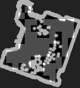
Figure 7:Downsampled free-space grid used to construct the spanning tree graph.
A degree first search (DFS) is conducted over the free cells, from which sparse waypoints are created.
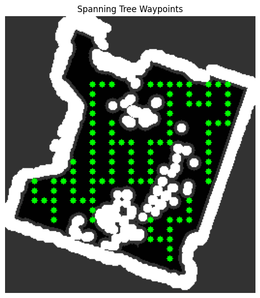
Figure 8:Depth-first search spanning tree generated over the free-space grid.
A black image, of the same resolution as the original costmap is then created and white squares, with half the cell width, are placed in the center of each cell and in between each cell. Waypoints are created from the contours of this tree. These waypoints represent a circumnavigation around the DFS tree.
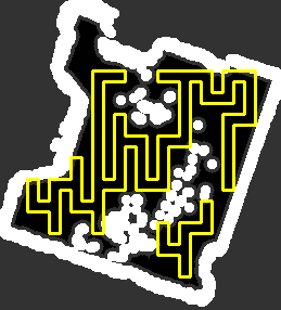
Figure 9:Coverage waypoints generated by tracing the contour around the spanning tree structure.
A segment from this circumnavigation is then removed from the path
Source
%matplotlib widget

interactive_path_slider('figures/navigator_results/Initial_Costmap.png',
                        'figures/navigator_results/spanning_tree_path.csv',
                        "Spanning Tree Path Viewer",
(255, 0, 0), 1)A lab cleanup robot must not blindly follow waypoints. If it does it might collide with obstacles near the map boundary or collide with moving objects.
Nav2 implements several low level real-time trajectory planners that plan inside the live updating costmap Macenski et al., 2023. They handle how the waypoints are followed and how much influence the map ought to have on the generated trajectory. The system described in this section implements an MPPI controller Williams et al., 2017 due to its superior performance in highly dynamic environments, like labs where students or people frequently walk Elbouhy et al., 2024. Other planners that were considered include DWB (Dynamic Window Approach Behavior-based) Thrun et al., 1997 and RPP (Regulated Pure Pursuit) Macenski et al., 2023.
- Macenski, S., Martín, F., White, R., & Ginés Clavero, J. (2020). The Marathon 2: A Navigation System. 2020 IEEE/RSJ International Conference on Intelligent Robots and Systems (IROS). https://github.com/ros-planning/navigation2
- Becoy, A. J., Khomenko, K., Peternel, L., & Rajan, R. T. (2025). Autonomous navigation of quadrupeds using coverage path planning with morphological skeleton maps. Frontiers in Robotics and AI, Volume 12-2025. 10.3389/frobt.2025.1601862
- Niu, H., Ji, X., Zhang, L., Wen, F., Ying, R., & Liu, P. (2025). A Skeleton-Based Topological Planner for Exploration in Complex Unknown Environments. https://arxiv.org/abs/2412.13664
- Gabriely, Y., & Rimon, E. (2001). Spanning-tree based coverage of continuous areas by a mobile robot. Proceedings 2001 ICRA. IEEE International Conference on Robotics and Automation (Cat. No.01CH37164), 2, 1927–1933 vol.2. 10.1109/ROBOT.2001.932890
- Macenski, S., Moore, T., Lu, D. V., Merzlyakov, A., & Ferguson, M. (2023). From the desks of ROS maintainers: A survey of modern & capable mobile robotics algorithms in the robot operating system 2. Robotics and Autonomous Systems, 168, 104493. 10.1016/j.robot.2023.104493
- Williams, G., Aldrich, A., & Theodorou, E. A. (2017). Model Predictive Path Integral Control: From Theory to Parallel Computation. Journal of Guidance, Control, and Dynamics, 40(2), 344–357.
- Elbouhy, S. M., Adamanov, A., Braun, P. M., & Rose, H. W. (2024). Comparative Analysis of Local Trajectory Planning Algorithms in ROS2. Hamburg University of Technology.
- Thrun, S., Fox, D., & Burgard, W. (1997). The dynamic window approach to collision avoidance. IEEE Robotics & Automation Magazine, 4(1), 23–33.
- Macenski, S., Singh, S., Martin, F., & Ginés Clavero, J. (2023). Regulated Pure Pursuit for Robot Path Tracking. Autonomous Robots, 47(6), 685–694. 10.1007/s10514-023-10097-6